Heat conduction

Node.js examples of heatConduction, in examples/heatConduction. Run the commands below from that folder (see running an example). All results are from FEAScript-core 0.4.0.

Wall in 1D

Steady heat flow through a building wall 0.15 m thick. The inner side exchanges heat with the room by convection ($h = 1$ W/(m²·K), $T_\infty = 25$ °C) and the outer side is held at 5 °C. $k = 1$ W/(m·K).

node heatConduction1DWall/heatConduction1DWall.js

Source: heatConduction1DWall.js

Geometry

Mesh

Results

With constant $k$ and no heat source the temperature is linear through the wall. It falls from 7.6087 °C at the inner side to 5 °C at the outer side, the exact values: the heat flux is $(25 - 5) / (1/h + W/k) = 17.3913$ W/m², so $T(0) = 25 - 17.3913 / h$. The example solves with the Jacobi method; the linear elements are exact at the nodes. The example prints the node coordinates and the solution vector.

Bi-material wall in 1D

The same wall in two layers: concrete ($k = 10$ W/(m·K)) for $x < 0.075$ m and insulation ($k = 1$ W/(m·K)) beyond. The conductivity is given as a function of position, (x) => (x < 0.075 ? 10 : 1). The inner side exchanges heat by convection ($h = 25$ W/(m²·K), $T_\infty = 5$ °C) and the outer side is held at 20 °C.

node heatConduction1DWall/heatConduction1DVaryingK.js

Source: heatConduction1DVaryingK.js

Geometry

Mesh

Results

The heat flux is the same in both layers, so the temperature gradient is 10 times steeper in the insulation. The temperature is 9.8980 °C at the inner side and 10.8163 °C at the interface. The example prints the node coordinates and the solution vector.

Fin in 2D

A 4 m × 2 m cooling fin, $k = 1$ W/(m·K): fixed temperature of 200 °C at the bottom and right edges, symmetry at the left edge, and convection ($h = 1$ W/(m²·K), $T_\infty = 20$ °C) at the top edge. The mesh is generated by FEAScript.

node heatConduction2DFin/heatConduction2DFin.js

Source: heatConduction2DFin.js

Geometry

Mesh

Results

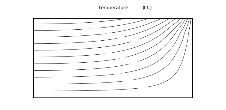
The lowest temperature, 81.3187 °C, is at the top left corner, farthest from the heated edges. The example prints the node coordinates and the solution vector.

Comparison with Elmer

The fin was also solved with Elmer, the open-source finite element software of CSC – IT Center for Science, on the same structured meshes, with linear and quadratic quadrilaterals from 231 to 51,681 nodes. The problem has an exact solution, a Fourier series,

$$T(x, y) = 200 + \sum_{n=1}^{\infty} A_n \cos(\lambda_n x) \sinh(\lambda_n y), \qquad \lambda_n = \frac{(2n-1)\pi}{8},$$

so both programs are compared with it at every node, and with each other:

Elements	Mesh	Nodes	Largest error (°C)	RMS error (°C)	Difference from Elmer (°C)
Linear	20 × 10	231	1.0e0	1.1e-1	3.1e-13
Linear	40 × 20	861	5.7e-1	3.2e-2	3.4e-12
Linear	80 × 40	3,321	3.1e-1	8.8e-3	9.2e-12
Linear	160 × 80	13,041	1.6e-1	2.4e-3	4.4e-11
Linear	320 × 160	51,681	8.1e-2	6.7e-4	1.9e-10
Quadratic	10 × 5	231	8.0e-1	6.7e-2	5.4e-13
Quadratic	20 × 10	861	3.9e-1	1.7e-2	2.5e-12
Quadratic	40 × 20	3,321	2.0e-1	4.3e-3	6.3e-12
Quadratic	80 × 40	13,041	9.7e-2	1.1e-3	2.9e-11
Quadratic	160 × 80	51,681	4.9e-2	2.7e-4	1.0e-10

The errors of Elmer are the same to the digits shown, and the temperatures of the two programs differ by at most 1.9e-10 °C on every mesh, the round-off of double precision arithmetic, which grows with the size of the mesh. The largest error is at the node next to the top right corner, where the fixed temperature of the right edge meets the convection of the top edge and the exact solution is not smooth. There it falls only in proportion to the element size $h$, with either element; the RMS error over all the nodes falls about as $h^2$.

FEAScript-core 0.4.0 was used, with "frontal" and "lusolve", which give the same temperatures. Elmer used its HeatSolver with the UMFPACK direct solver, run on one core as a single MPI process. For the solve times, see Solvers. The benchmark, with the Elmer setup, is in FEAScript-benchmark.

Comparison with scikit-fem

The fin was also solved with scikit-fem, an open-source finite element library for Python, on the same meshes, with the same elements and its default direct solver. The temperatures of FEAScript and scikit-fem differ by at most 1.7e-10 °C on every mesh, from 231 to 51,681 nodes, as close as with Elmer.

Fin in 2D, Gmsh mesh

The fin of the previous example on an unstructured mesh made with Gmsh, read from rect_quad.msh (see Gmsh import). The geometry and boundary conditions are the same; the physical groups of the mesh are tagged bottom, left, top, right, like the sides of the structured mesh.

node heatConduction2DFin/heatConduction2DFinGmsh.js

Source: heatConduction2DFinGmsh.js

Mesh

Results

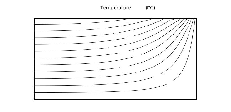
The lowest temperature is 81.3207 °C, against 81.3187 °C on the structured mesh. The example prints the node coordinates and the solution vector.

Comparison on unstructured meshes

The fin was also solved with Elmer and scikit-fem on 16 unstructured meshes made with Gmsh, read by all three programs: linear and quadratic triangles and quadrilaterals, up to 89,209 nodes. The temperatures of FEAScript and scikit-fem differ by at most 1.1e-10 °C when scikit-fem uses the same Gauss rules, and those of FEAScript and Elmer by at most 2.8e-11 °C.

On a distorted quadrilateral, these rules do not integrate exactly: FEAScript uses 2 × 2 points on linear elements and 3 × 3 on quadratic ones. With a much finer rule in scikit-fem, the RMS error against the exact solution is only 1.2% to 2.1% lower. On triangles with straight sides, the rules are exact. The benchmark is in FEAScript-benchmark.

Rhomboid fin in 2D, Gmsh mesh

A fin whose top edge is shifted by 1 m, so the left and right edges slant. The boundary conditions are those of the rectangular fin. The mesh is read from rhom_quad.msh.

node heatConduction2DFin/heatConduction2DRhomFinGmsh.js

Source: heatConduction2DRhomFinGmsh.js

Geometry

Mesh

Results

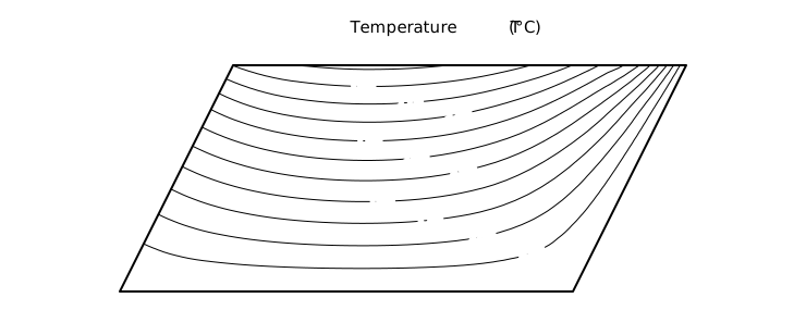
The lowest temperature, 87.5205 °C, is on the top edge, at $x = 2.25$ m, between two nodes (the lowest nodal value is 87.6060 °C, at $x = 2.3333$ m). The example prints the node coordinates and the solution vector.

Fin in 2D with spatially varying k and Q

The fin of the first 2D example with two materials and a local heat source: $k = 10$ W/(m·K) for $x < 2$ m and $k = 1$ W/(m·K) beyond, and a heat source $Q = 500$ W/m³ in the strip $y > 1.5$ m. Both are given as functions of position.

node heatConduction2DFin/heatConduction2DVaryingKQ.js

Source: heatConduction2DVaryingKQ.js

Geometry

Mesh

The mesh is that of the fin in 2D: 8 × 4 quadratic quadrilaterals.

Results

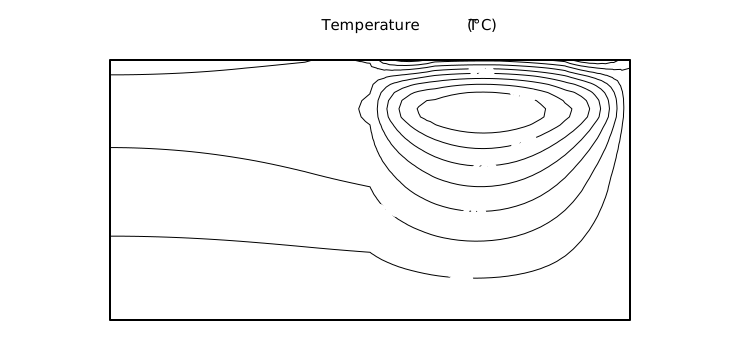
The heat source raises the temperature above that of the heated edges. The highest temperature, 240.1414 °C, is at (2.875 m, 1.625 m), inside an element, in the low-conductivity half, where the heat has the most difficulty escaping. The highest nodal value is 237.4724 °C, at (3 m, 1.5 m). On a mesh refined 8 times in each direction (64 × 32 elements) the peak is 240.2033 °C at (2.875 m, 1.594 m).

At $x = 2$ m the contour lines bend: the heat flux is continuous across the material interface, so the temperature gradient is 10 times steeper on the low-conductivity side.